System Design Advanced
Proximity Search
A rider opens the app at rush hour. Matching needs drivers within about 2 km, not every driver in the city sorted by age or ID. Databases are excellent at one-dimensional ranges. Two coordinates and a radius are a different problem.
Proximity search shows up whenever you query by location: nearby drivers, restaurants, people, or devices. The hard part is not distance math. It is getting a that preserves enough two-dimensional closeness to avoid a full table scan, then finishing with a and a .
What happens first?
Why plain indexes fail
Lat or lng alone is a strip, not a neighborhood of nearby points.
Pick a family
Spatial tree for shapes, or encoded cells for moving points.
Index narrows the map to a small local patch of rows.
Exact distance or geometry runs only on that handful.
Try it: geohash candidates then distance rank
Proximity search usually has two stages: a cheap spatial index (here, geohash prefixes) to gather candidates, then an exact distance filter and sort. Changing precision trades recall for scan size.
- Query geohash
- tdr1v
- Prefix candidates
- 5
- In radius
- 4
- Radius km
- 3
Results inside radius (sorted)
haversine- Cafe A0.00 km · tdr1v
- Cafe B0.70 km · tdr1v
- Park1.06 km · tdr1v
- Bookstore1.68 km · tdr1y
Index stage
geohashPrefix lookup gathers candidates from a sorted keyspace or reverse index. Quadtrees and S2 cells play the same role.
Refine stage
distanceExact meters filter false cell neighbors. Production systems also query adjacent cells when the point sits near a border.
Scale
shardingHot downtown cells need sharding or denser precision. Airport-scale radii may fan out to many cells on purpose.
Move the query point and radius. Geohash prefixes candidate-filter the map so you do not scan every place, then haversine ranks true distance.
Never return raw prefix matches alone. Hash cells are squares on a sphere approximation. Always apply a true distance check (haversine or projected meters) before showing “near me” results.
What actually happens
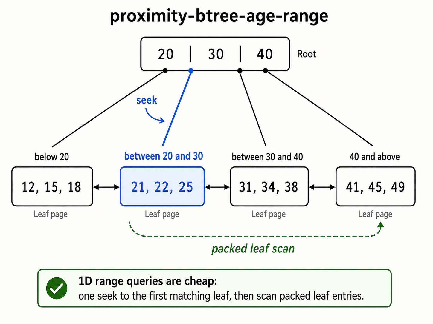
Ask for users aged 20 to 25 and a wins: those keys sit packed on disk pages. One seek, then a short sequential read. Age filters feel instant because consecutive ages share the same leaves.
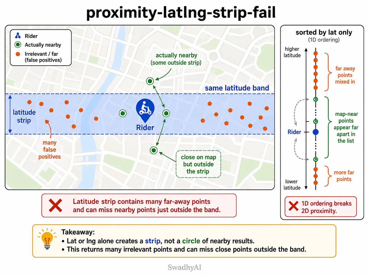
Ask for every driver within 2 km and the same database may fall apart. Latitude and longitude are two numbers. A single B-tree sorts one key at a time. Index latitude and you get a horizontal strip. Index longitude and you get a vertical strip. A composite (lat, lng) still sorts primarily by the first column, so the "strip" can still hold millions of rows with no distance ranking.
The naive recovery is brute force: compute distance for every row and discard anyone past 2 km. Correct, and hopeless at city scale. A exists to produce a cheap , then you with exact math (haversine or a geometry predicate). The index may over-approximate with cells or boxes, but it must never silently drop a true neighbor your query promises.
How to choose an approach
Once you see why a plain cannot keep map neighbors together, three questions pick the right family.
1. Are you indexing shapes? Polygons, roads, delivery zones, containment, and intersection need a custom spatial tree (PostGIS / GiST style, or Elasticsearch geo via ideas).
2. Are you indexing moving points? Drivers, devices, and live users want cheap writes. Encode each location into a cell ID (, , ) and use an ordinary sorted index or hash lookup.
3. Will you always post-filter? If your design ends at WHERE geohash LIKE 'dr5ru%' without exact distance, boundary and corner errors will ship to production.
Rule of thumb
Spatial tree for shapes. Encoded cells for moving points. Always finish with a on the . The index is a filter for "maybe nearby," not the final ranking authority.
From problem to mechanism
Here is the rush-hour matching story slowed down, so you can see where the naive approach fails and what the fix changes.
Problem. Match a rider to drivers within about 2 km. Positions update constantly. Latency must stay interactive while the city has hundreds of thousands of online drivers.
Naive system. Index latitude (or a composite lat/lng) on a , or scan every row and compute distance. The strip still holds faraway false positives; brute force does 2×10⁵ distance computations per request in a city with 200,000 online drivers.
Break it. A geohash-only query without a neighbor ring misses the nearest driver sitting 10 m across a cell edge. Product shows "no drivers" while someone is meters away. Skipping exact distance also ranks corner points that sit outside the real radius.
Mechanism. Use a (custom tree or encoded cell key) to produce a small local , then with haversine or geometry. If a ring yields about 400 candidates, you cut work by roughly 500× before ranking, then still pay exact math on those 400 (see Numbers to know below).
Why one dimension cannot keep 2D neighbors
The mechanism assumes you already believe a one-key index cannot preserve map closeness. Start with ages, which databases already do well, then contrast that with latitude: same engine, same table size, very different outcome.
Age range (works)
Keys 20, 21, 22… pack together. "Between 20 and 30" is a contiguous leaf walk on a .
Lat/lng (breaks)
Flatten the map to one sorted axis and ground neighbors can land far apart in the index. Closeness is not a 1D interval anymore.
Read the age B-tree like a story. The root says where ages live. For “everyone between 20 and 30,” the engine seeks once into the leaf that starts that range, then walks packed siblings. That is why age filters feel instant.
Now put a rider on the map and index latitude alone. The query becomes a horizontal strip: same latitude band, any longitude. Far orange dots ride along inside the strip, while a truly nearby green pin can sit just outside the band. On the right, sorting by latitude only makes map-neighbors look far apart in the list.
Family 1: custom spatial trees
After the strip failure, the first recovery family keeps spatial locality inside the tree shape. On disk, the winners behave like : balanced depth, page-sized nodes, predictable I/O.
A quadtree recursively divides a region into four quadrants. Dense quadrants split further, so a busy city receives finer cells than empty countryside. A radius query traverses every node whose bounding region intersects the search circle; it cannot simply visit the rider’s leaf and assume a fixed number of adjacent leaves is enough. At the leaves, exact distance checks discard the points that lie in an intersecting rectangle but outside the circle.
Follow the left map first. Sparse NW, NE, and SW stay coarse. The dense SE keeps splitting until every leaf holds at most k = 5 points. The right side is the same story as a tree: only overloaded cells grow children.
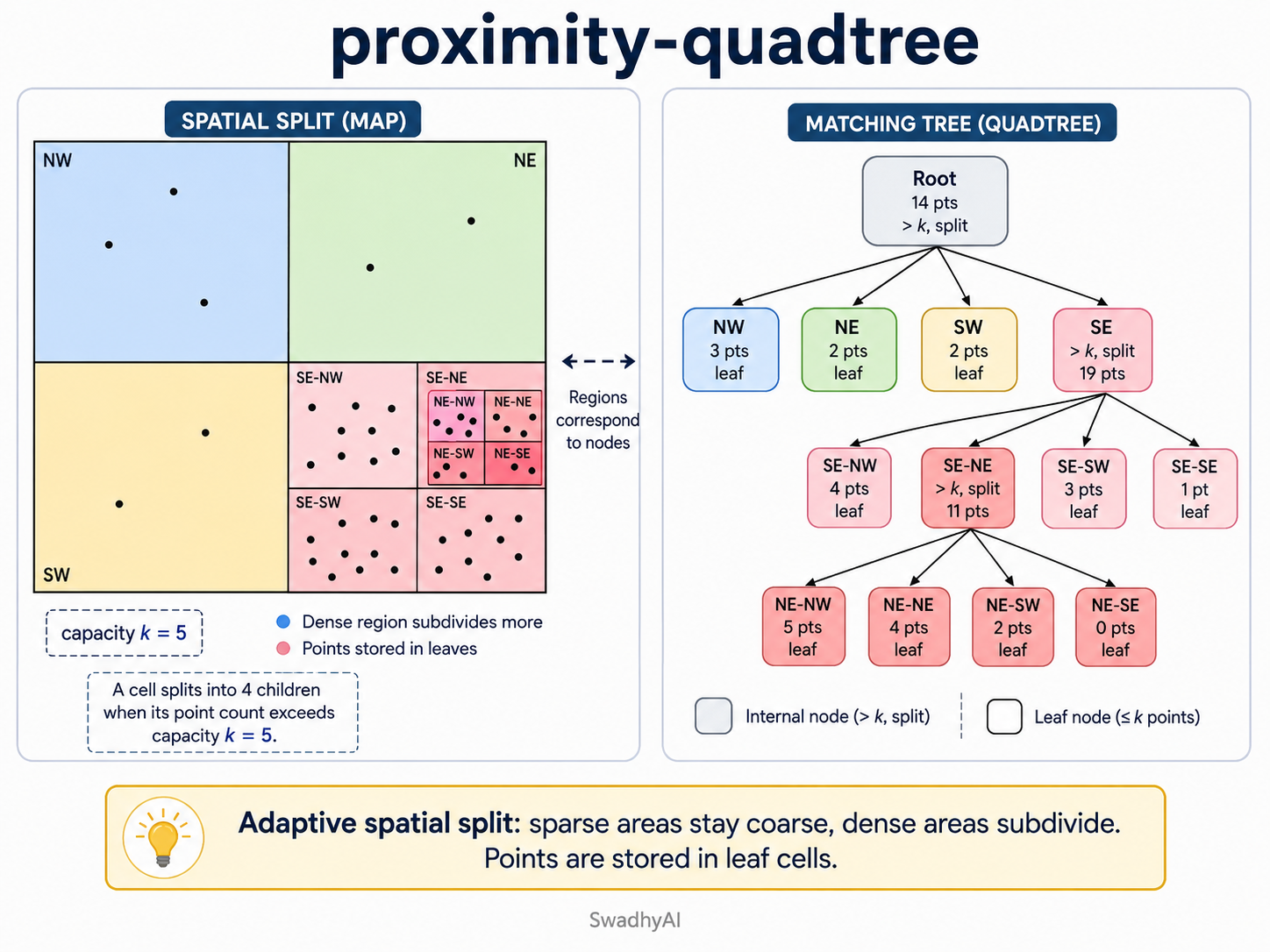
That density adaptation is the gift. The cost at database scale is uneven depth (busy downtowns go deepest) and pointer chasing that turns into random disk reads once the tree no longer fits in RAM. Quadtrees stay common in memory for map tiles and games. They are a weak default for a mutable on-disk primary index.
and
A k-d tree partitions points by alternating coordinate axes. Balanced median splits keep the tree shallow for a reasonably static dataset, while bounding regions help prune subtrees that cannot intersect the query. Frequent updates can disturb the balance and require maintenance or rebuilding. The key question is how many tree regions a real query touches, because logarithmic depth alone does not imply logarithmic work for every radius search.
Classic k-d trees share the disk problem: pointers. The modern packaging is the BKD tree: pack points into page-sized blocks, often rebuild from batches. That is the lineage behind Elasticsearch geo fields. Great for chunked/immutable-ish data; less natural for millions of single-point rewrites per second.
Wrap every object in a . Nest nearby rectangles inside larger ones up to the root. Leaves share depth; nodes fit pages; inserts/deletes split and merge like a B-tree.
Rectangles may overlap, so a query can descend multiple branches. R*-tree heuristics keep overlap low in real systems. PostGIS (GiST), SQLite, and Oracle Spatial lean on this family when you need "does this zone contain this address" or "does this road cross this county."
Family 2: encoded keys on ordinary indexes
Custom trees are not the only path. For moving points you can skip the custom tree and flatten each location into a cell ID a normal , hash index, or sorted set already understands.
Hierarchical grid: each character (5 bits) zooms into one of 32 subcells. Shared prefixes usually mean shared cells. A five-character geohash is roughly kilometers across; nine characters lands near meters. Redis GEOADD stores a 52-bit geohash integer as a sorted-set score.
Walk left to right. Layer 1 picks a coarse cell. Layer 2 zooms inside it. Layer 3 is fine enough to mark a city. Pune’s real hash looks like te7x2, but the idea is the same: longer shared prefixes mean a smaller shared box on the map.
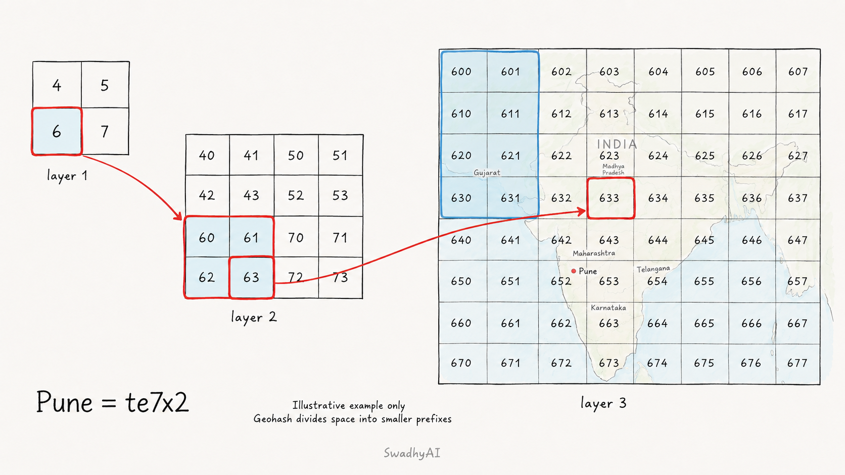
Cell boundaries are the main correctness trap. Two points a meter apart may have unrelated prefixes because one lies across an edge. Enumerate every cell that intersects the requested radius, fetch candidates from those cells, and apply the final distance predicate. A fixed 3×3 neighborhood is sufficient only when the chosen cell dimensions and query radius make it cover the whole circle. Larger radii, high latitudes, and changing resolution can require more cells.
-- candidates from a prefix (still over-approximate)
SELECT id FROM drivers
WHERE geohash LIKE 'dr5ru%'   -- plus neighbor prefixes in app code
-- then: filter by ST_Distance / haversine < 2000m and rankand
S2 maps the sphere onto cube faces and recursively subdivides them into hierarchical cells with 64-bit identifiers. Its region-covering operations can approximate a spherical query with a bounded set of cells, which is useful around the antimeridian and at global scale. The cells are not perfectly equal-area, and a cover can include extra ground area. Query the cover, then evaluate the actual spherical geometry to remove those extra candidates.
H3 provides a hierarchical grid made mostly of hexagons, with pentagons required by the spherical layout. A cell identifier is useful for aggregation and neighbor traversal, but graph distance in cells is not the same as a fixed distance in meters. Use the library’s supported traversal and covering behavior, handle distortion near exceptional cells, and choose enough cells for the requested geographic radius before exact filtering.
Which should you use?
With both families in view, this table is the decision aid, plus the scale numbers that make the candidate-and-filter path worth it.
| When | Reach for | Trade-off |
|---|---|---|
| Polygons, roads, zones, containment | / PostGIS GiST (or ES for geo fields) | Rich geometry; writes and rebalance cost more |
| Moving points, high update rate | / / on ordinary indexes | Cheap updates; mostly points; always ring + post-filter |
| In-memory tiles / games | (or grid hash) | Simple; not your default durable DB index |
Numbers to know
- About 200,000 online drivers: brute force does 2×10⁵ distance checks per request.
- If a complete cell cover returns 400 candidates from a city with 200,000 drivers, exact-distance evaluations drop by a factor of 500 for that query. This is an illustrative workload, not a guaranteed property of geohash. Dense downtown cells may contain many more points. Measure candidate counts by region and radius, adapt resolution where useful, and cap requests whose radius would effectively scan the city.
- At 5,000 match requests/s, that gap decides melting the fleet versus staying interactive.
Failure timeline, and what still breaks after the fix
Putting the pieces together, here is how a cell-boundary miss plays out, then the ways an improved design can still go wrong.
Timeline: the boundary miss
- Rider sits on the edge of cell
dr5ru. - Nearest driver is 10 m away in neighbor
dr5rg. - Naive
LIKE 'dr5ru%'returns empty; product shows "no drivers." - Fix: query all cells intersecting the radius (a 3×3 ring only when it fully covers the circle), by exact meters, then rank. Index over-approximates; distance restores truth.
Still fails when…
- You skip the neighbor ring and miss true neighbors across a cell edge.
- You rank by cell alone; square corners can sit outside the real radius.
- You use a on disk for high-churn driver updates.
Trade-offs
- handle rich geometry, but writes and rebalance cost more.
- Encoded cells update cheaply for points, yet always need ring plus .
- suits chunked geo fields, not millions of single-point rewrites.
Wrap-up
You have seen the strip failure, both index families, and the boundary miss. Use these exercises to check the ideas stuck, then follow the primary sources.
Exercises
- Latitude strip. Why does a on latitude alone fail for "drivers within 2 km"? Give the strip argument, not "B-trees cannot do ranges."
- Edge rider. A rider sits on a edge. Sketch the complete cell-cover query, state when 3×3 is sufficient, and explain what removes from the corner cells.
- 50k updates/s. Dispatch updates 50,000 driver positions/s. Would you pick PostGIS updates or cell IDs on a sorted index? Defend with write cost and query shape.
Primary sources
- Guttman, A. R-Trees: A Dynamic Index Structure for Spatial Searching (SIGMOD 1984).
- Uber Engineering: H3 documentation.
- RFC 7946: GeoJSON (geometry interchange; pairs with PostGIS / GIS stacks).
- Google S2 Geometry Library documentation (spherical cells and hierarchical IDs).
Key takeaway
Proximity is hard because one-dimensional sort order cannot preserve two-dimensional closeness. Recover locality with a spatial tree or an encoded cell key, generate a small , then finish with exact distance or geometry. Name the library if you know it; the candidate-and-post-filter reasoning is what shows you understand the problem.
Practice and further reading
Use these exercises to connect the lesson to a design decision. State your assumptions, trace what happens to one request, and explain the rule that must remain true even during a failure. That rule is the design's correctness invariant.
Focus for this lesson: Explain why 1D indexes fail on lat/lng, then choose spatial trees vs encoded cells, generate a candidate ring/box, and always post-filter with exact distance or geometry.
Explain the decision
Why does a B-tree on latitude alone fail for “drivers within 2 km”?
Read the reasoning
It selects a horizontal strip of Earth that can still hold huge row counts with no distance ranking, so the engine falls back toward scanning and per-row distance.
Apply it to a production scenario
A rider sits on a geohash cell edge and a naive prefix query returns no drivers. What failed?
Read one approach
Boundary straddle: the nearest driver lived in a neighbor cell. Query the ring of neighbors, then post-filter by exact meters.
Work through the numbers
200,000 online drivers; a cell ring yields 400 candidates. Roughly how much work did the index remove before exact distance?
Read the worked calculation
About 500× fewer distance computations per request (2e5 → 4e2), before ranking.
Reason through a failure
What must the spatial path preserve?
Read the recovery reasoning
No true neighbor inside the stated radius/geometry contract is dropped by the candidate generator; over-approximation is allowed, under-approximation is not.
Sources and further study
- Guttman — R-Trees: A Dynamic Index Structure for Spatial Searching
- Uber H3 documentation
- Google S2 Geometry Library
- RFC 7946 — GeoJSON
Continue with Distributed Hash Tables.